User Manual
Overview
Below are the ROS topics of each sensor modality in INS. Please click on the link on each message type for their detailed definition. Other details such as resolutions are also provided. The naming convention `/<hardware-unit>/<modality>/…' is applied for all topics.
| Modality | Hardware | ROS topics / Sensor suite | Message type | Rate (Hz) | Notes |
|---|---|---|---|---|---|
| Camera | D435i | /d435i/depth/image_raw /d435i/infra1/image_rect_raw /d435i/infra2/image_rect_raw /d435i/color/image_raw | sensor_msgs/Image | 30 | 848 x 480 Greyscale 1280×720 Greyscale 1280×720 Greyscale 1280×720 RGB |
| D455 | /d455/depth/image_raw /d455/infra1/image_rect_raw /d455/infra2/image_rect_raw /d455/color/image_raw | 30 | 848 x 480 Greyscale 1280×720 Greyscale 1280×720 Greyscale 1280×720 RGB | ||
| IMU | D435i | /d435i/imu | sensor_msgs/Imu | 400 | Bosch BMI055 |
| D455b | /d455b/imu | 400 | See datasheet | ||
| Livox Mid 360 | /livox/lidar/imu | 400 | See datasheet | ||
| Lidar | Livox Mid360 | /livox/lidar | livox_ros_driver/CustomMsg | 10 | 1 channel. Points per channel: 9984 Point format: see our manual |
Depth data
We provide two types of depth data. One is directly observed by the RealSense sensor, which has very low quality. The other is a dense, high-precision depth obtained by projecting the ground truth point cloud and completing the depth, which requires the ground truth pose and can only be generated after the LiDAR is activated. As a result, the first 8 frames of the depth projection data are missing. Users can either use the raw depth data or the data after the 8th frame.
Lidar data
Resolution and rate
In all sequences, the mid70 Livox lidar have one single non-repetitive line with 9984 points per line. All lidars output data at 10 Hz.
Point format
For livox lidar, the point has a custom structure that is defined by the manufacturer as follows:
# Livox costum pointcloud format.

uint32 offset_time      # offset time relative to the base time
float32 x               # X axis, unit:m
float32 y               # Y axis, unit:m
float32 z               # Z axis, unit:m
uint8 reflectivity      # reflectivity, 0~255
uint8 tag               # livox tag
uint8 line              # laser number in lidar
Please follows the instructions here to install the livox driver, after which you should be able to import and manipulate the livox message in ROS python or C++ program.
Time stamp
For INS Dataset, please take note of the following:
- For the ouster data, the timestamp in the message header corresponds to the end of the 0.1s sweep. Let us denote it as \(t_h\). Each lidar point has a timestamp (in nanosecond) that is relative to the start of the sweep, denoted as \(t_r\). The absolute time of the point \(t_a\) is therefore:
- For the livox data, the timestamp in the message header corresponds to the start of the 0.1s sweep. We us denote it as \(t_h\). Each lidar point has a timestamp (in nanosecond) that is relative to the start of the sweep, denoted asc \(t_r\). The absolute time of the point \(t_a\) is therefore:
Coordinate systems
The main coordinate systems in INS Dataset is defined as follows:
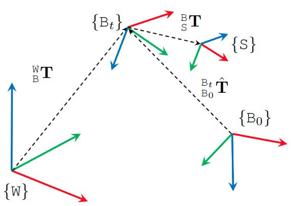
First, the coordinate system of the prior maps is referred to as the World frame \(\mathtt{W}\). Then the Body frame \(\mathtt{B}\) coincides with the VN100 IMU in the NTU sequences, and the VN200 in the KTH and TUHH sequences. Each sensor has a Sensor frame \({\mathtt{S}}\) attached to it.
The extrinsics of the sensors in INS are declared as transformation matrices \({}^{\mathtt{B}}_{\mathtt{S}}\bf{T} = \begin{bmatrix} {}^{\mathtt{B}}_{\mathtt{S}}\mathrm{R} & {}^{\mathtt{B}}_{\mathtt{S}}\mathrm{t} \\ 0 &1\end{bmatrix}\), where \({}^{\mathtt{B}}_{\mathtt{S}}\mathrm{R}\) and \({}^{\mathtt{B}}_{\mathtt{S}}\mathrm{t}\) are respectively the rotational and translational extrinsics.
Therefore if one observes a landmark \({}^{\mathtt{C}}\mathrm{f}\) in the camera frame \(\mathtt{C}\), its coordinate in the body frame \({}^{\mathtt{B}}\mathrm{f}\) is calculated as:
\[{}^{\mathtt{B}}\mathrm{f} = {}^{\mathtt{B}}_{\mathtt{C}}\mathrm{R} {}^{\mathtt{C}}\mathrm{f} + {}^{\mathtt{B}}_{\mathtt{C}}\mathrm{t}\]The ground truth data in our csv files are the poses \(({}^{\mathtt{W}}_{\mathtt{B}_t}\mathrm{q}, {}^{\mathtt{W}}_{\mathtt{B}_t}\mathrm{p})\), where \({}^{\mathtt{W}}_{\mathtt{B}_t}\mathrm{q}\) and \({}^{\mathtt{W}}_{\mathtt{B}_t}\mathrm{p}\) are the orientation (in quaternion) and position of the body frame at time t relative to the world frame.
In most cases, the SLAM estimate \({}^{\mathtt{B}_0}_{\mathtt{B}_t}\hat{\bf{T}}\) is relative to the coordinate frame that coincides with the body frame at initial time. It is therefore neccessary to align the SLAM estimate with the groundtruth. The evo package is a popular tool for this task.