Groundtruth
Below we provide more information on our groundtruth data.
Survey-grade prior map
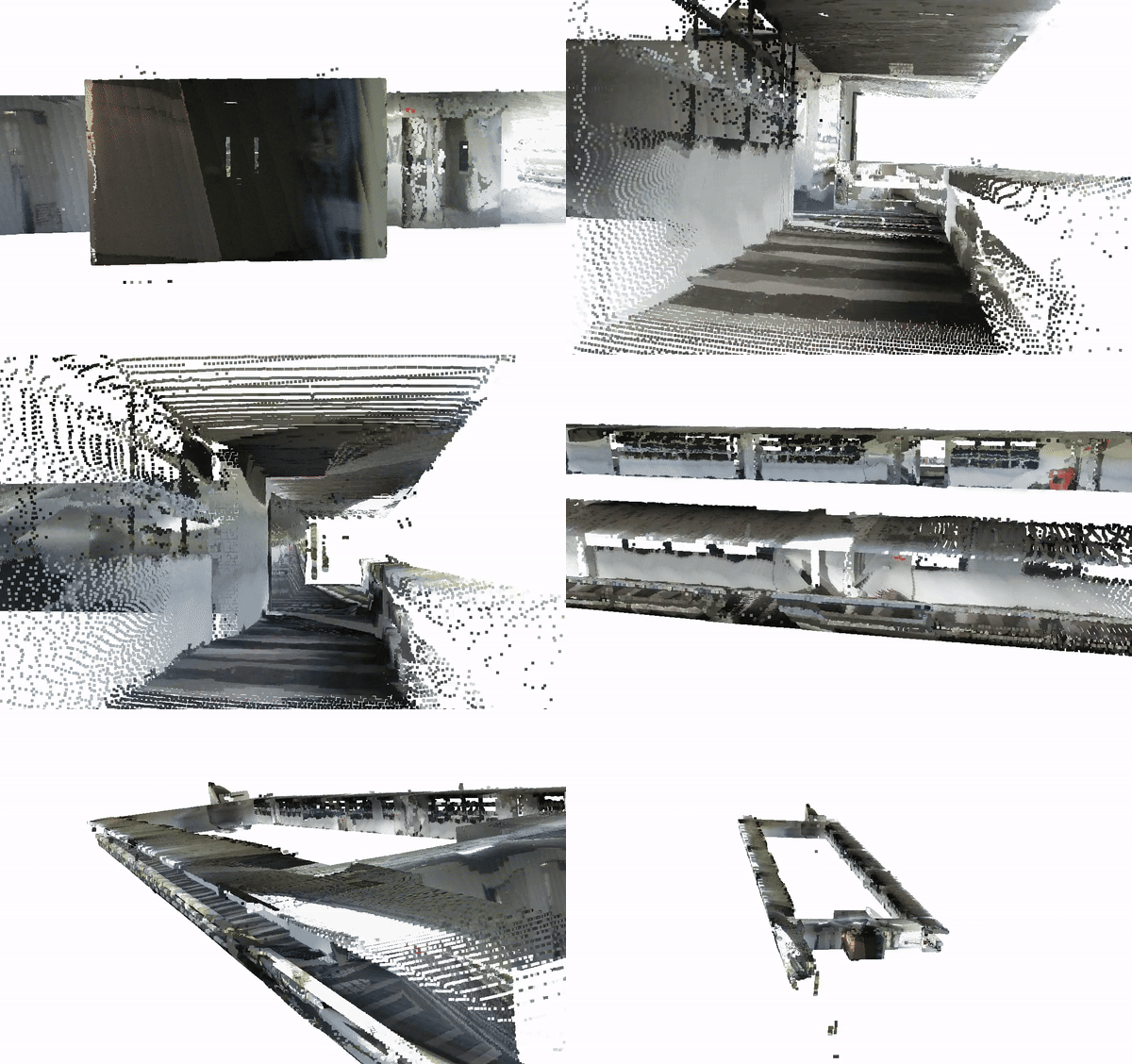
All ground truths ultimately come from the high accuracy survey-grade prior maps. You can download the original scans via the links below (please use CloudCompare to read the files):
 |  |  |
|---|---|---|
| Pointcloud Download Mesh Download | Pointcloud Download Mesh Download | Pointcloud Download Mesh Download |
Descrete time ground truth
For those who only need a traditional discrete-time ground truth for benchmarking SLAM methods, you can use the pose.txt associated with each sequence. The content looks like the following:
num	t                 x                 y                 z                 qx                  qy                 qz                  qw
11	1644823132.49211  49.2606317111444  107.371797989247  7.63580957239259  0.936118452267473  -0.351663294301812  0.003894594980225  -5.3806028052E-05
12	1644823132.59122  49.2617548510814  107.371820422962  7.63634221875222  0.936400655699795  -0.350853723839147  0.001952716665257  -0.007187723619002
13	1644823132.69085  49.2627442641658  107.370734597833  7.63708972884333  0.937130644015062  -0.348934531427190  0.005541781558079  -0.000370786684933
14	1644823132.79213  49.2634361009274  107.369692804349  7.63756375797164  0.935347736233029  -0.353687216878511  0.004396339541646  -0.003261462726211
15	1644823132.89130  49.2637252742628  107.368872120271  7.63750418262036  0.936261362661676  -0.351231145451445  0.005677919353789  -0.004370867600258
...
Here, num is the index of the lidar pointcloud in the bag file, t is the time stamp, and (x, y, z, qx, qy, qz, qw) is the pose of the body frame wrt to the world frame.
Continous-time ground truth
We generate the continous-time ground truth trajectories using our previous work, CTE-MLO: A Continuous-time and Efficient Multi-LiDAR Odometry with Localizability-aware Point Cloud Sampling(T-FR 2025), which leverages high-precision prior maps for accurate trajectories. For more advance users that would like to study the motion distortion on lidar, you can use the spline.csv file provided in the same folder (if you are not familar with B-spline, we recommend the following paper for the detail description of B-spline based continuous-time trajectory representation ).
The CTE-MLO can be easily configured to perform localization on a pre-built map by setting use_prebuild_map: True in the .yaml. Don't forget to specify the path of the pre-built map by setting the offline_map_path in .yaml. The init_T in the .yaml file represents the initial pose of the first scan in the pre-build map, which can be obtained either from a ground truth trajectory or through point cloud registration between the first scan and the pre-built map. To facilitate registration, we provide a point cloud registration GUI.
Testing on MCD Prior Map:
source ~/ctemlo_ws/devel/setup.bash
roslaunch cte_mlo mapping_mcd_prior.launch
rosbag play ntu_day_01/ntu_day_01_mid70.bag
Remark: Please wait until the terminal displays The Pre-build Map has been Voxelized before playing the rosbag.
The control points of the spline are listed in this file. The content resembles the following:
Dt: 0.025, Order: 6, Knots: 24045, MinTime: 1644823132.49097, MaxTime: 1644823733.59097
0,1644823132.4909698963165283,49.2601663093799687,107.3714204060612047,7.6355324272268943,0.9350584912955798,-0.3544839325422865,-0.0006156075556602,0.0025259558046850
1,1644823132.5159699916839600,49.2604201766309515,107.3716637079355962,7.6356371447402402,0.9379846150800922,-0.3462143713078067,0.0005065405451423,-0.0178945351900358
2,1644823132.5409698486328125,49.2606213815611795,107.3717670418042047,7.6358132610019718,0.9354176646728326,-0.3532940094282990,0.0080878815549711,0.0105698482512218
3,1644823132.5659699440002441,49.2608259618997621,107.3719814523942944,7.6359423034838736,0.9358444686488053,-0.3522668912610597,-0.0027447487380264,-0.0097792727269988
4,1644823132.5909698009490967,49.2610915208195834,107.3720644627877050,7.6360616461728057,0.9361526518581488,-0.3515835046668936,0.0011728044948194,-0.0024240863675093
5,1644823132.6159698963165283,49.2614226852895811,107.3720311712474995,7.6362061007328341,0.9359967890920514,-0.3519082642918072,-0.0015771747359690,-0.0082520816979596
...
The first line lists the parameters of the spline: the knot length Dt, the spline Order, the number of Knots, the starting time MinTime and the ending time MaxTime of the trajectory. Subsequently, the index, time stamp and the value of each control pose (x,y,z,qx,qy,qz,qw) is listed line by line.
The best way to read and query the spline information is by using the package ceva that is a python wrapper for the basalt library. For example one can create a spline from the log file as follows:
import numpy as np

from ceva import Ceva

spline_log = '../example/spline.csv'

def load_spline(x):

    # Read the spline
    log = open(x, 'r')

    # Extract some settings in the header
    log_header = log.readline()
    log.close()

    # Read the dt from header
    dt = float(log_header.split(sep=',')[0].replace('Dt: ', ''))
    # Read the order
    order = int(log_header.split(sep=',')[1].replace('Order: ', ''))
    # Read the knots
    knots = int(log_header.split(sep=',')[2].replace('Knots: ', ''))
    # Read the start time in header
    start_time = float(log_header.split(sep=',')[3].replace('MinTime: ', ''))
    # Calculate the end time
    final_time = start_time + dt*(knots - order + 1)

    # Create the spline from text
    knots = np.loadtxt(x, delimiter=',', skiprows=1)
    spline = Ceva(order, dt, start_time, x)

    return spline

# Load the spline
gt_traj = load_spline(spline_log)

# Sample the pose at 100s after the start
pose_stamped = gt_traj.getPose(gt_traj.minTime() + 100) # Returns t, x, y, z, qx, qy, qz, qw
print(pose_stamped)

# You can also pass a vector of times and get an array
pose_stamped = gt_traj.getPose(gt_traj.minTime() + np.arange(0, 100, 0.1)) # Returns t, x, y, z, qx, qy, qz, qw
print(pose_stamped)